vol. 14 no. 1, March, 2009 Contents | Author index | Subject index | Search | Home

Term based comparison metrics for controlled and uncontrolled indexing languages

Introduction

We are in an era of a rapidly expanding number and diversity of systems for organizing information. Wikis, collaborative tagging systems and semantic Web applications represent broad categories of just a few emerging frameworks for storing, creating, and accessing information. As each new kind of information system appears, it is important to understand how it relates to other kinds of system. This understanding allows us to answer a variety of important questions, which will shape the way future systems are designed. Does the new system represent a less expensive way to achieve the same functionality as another? Might it be fruitfully combined with another approach? How similar is it to an exemplar in its domain?

In addition to deriving theoretical answers to questions at the level of the kind of system, such as, How does social tagging relate to professional indexing? (Feinberg 2006; Tennis 2006) or, How do the ontologies of computer science relate to the classifications of library and information science?, as addressed by Soergel (1999), it is also now of practical importance to find answers to specific instance-level questions. For example, Al-Khalifa and Davis (2007) attempt to answer the question, How do the tags provided by Delicious users relate to the terms extracted by the Yahoo indexing algorithm over the same documents? and Morrison (2008) asks, How do the results of searches performed on social tagging systems compare to those performed on full Web search engines? Answers to such questions provide vital knowledge to system designers, because, in the age of the Web, information systems do not operate in isolation from one another. It is both possible and beneficial to integrate components of different systems to create symbiotic aggregates that meet the needs of specific user groups better than any single system could, and doing so depends upon the knowledge of how the different systems relate. Would Yahoo automatic indexing be improved through incorporation of indexes provided by Delicious users? Comparative analyses of the components of the two systems can help tell us.

Both comparative studies of information systems in the abstract and efforts to design specific instances of new integrative systems can benefit from mechanisms that help to identify the specific similarities and differences that obtain between different systems. One facet of this is empirical, reproducible, quantitative methods of investigation. To inform both kinds of enquiry, empirical protocols that allow for reproducible, quantitative comparison would be beneficial. However, the term information system covers a vast and ill-defined set of things, each of which is composed of many complex components operating together in many different contexts to achieve a variety of different purposes. To conduct useful empirical comparisons of such systems, 1) hypotheses must be evaluated in light of the many contributing qualitative factors, and 2) reproducible metrics must be devised that can be used to test assumptions. While qualitative interpretations of the differences that hold between different kinds of information system continue to advance, there are few practical, reproducible metrics defined for use in empirical comparisons of system components.

Our broad goal in this work is to define a set of measurements, which can be taken of information systems, that are meaningful, widely applicable, and reproducible. The specific set of metrics introduced here do not intend nor pretend to be exhaustive nor definitive, in fact, we suggest that is not an attainable goal given the complexity of the systems under scrutiny. Rather, we advance them as an early set of candidates in what we expect will be a broad pool of metrics, which will continue to expand and be refined indefinitely. In light of these goals, the metrics defined here are meant for the characterization of one key component common to the vast majority of information systems in current operation, the language used to index the resources of interest within the system.

Zhang (2006:121) defines an indexing language as ‘the set of terms used in an index to represent topics or features of documents and the rules for combining or using those terms’. As the emphasis here is on empirical observation and many of the information systems under consideration offer little or no rules for the application nor of the construction of the terms, we will operate under the broader definition of indexing languages as sets of terms used in an index to represent topics or features. Notice that this definition spans both controlled languages, such as institutionally maintained thesauri, and uncontrolled languages, such as the sets of keywords generated by social tagging systems. Examples of indexing languages, as defined here, thus include the Medical Subject Headings (MeSH) thesaurus, the Gene Ontology as described by Ashburner et al. (2000), and the Connotea folksonomy as described by Lund et al. (2005). Each of these languages, though varying in relational structure, purpose, and application, is composed of a set of terms that represent aspects of the resources within the information systems that utilize them. Through comparisons of the features of these indexing languages, we hope to start work that will eventually allow us insight that will enable us to gain a better understanding not just of the relations between the languages, but, through them, of the relations between the systems that generate and use them.

In this work, we advance an approach to the automated, quantitative characterization of indexing languages through metrics based simply on the sets of terms used to represent their concepts. These metrics are divided into two groups, intra-set and inter-set. The intra-set metrics provide views on the shape of the sets of terms in aggregate. The inter-set metrics provide a coherent approach to the direct comparison of the overlaps between different term sets. The paper is divided into two main sections. The first section describes each of the metrics in detail and the second presents the results from a quantitative comparison of twenty-two different indexing languages. Results are provided for each language individually, using the intra-set metrics, and for each language pair, using the inter-set metrics. In addition to the broad all-against-all comparison, we present a more detailed exploration of the similarities and differences, revealed using the proposed metrics, that hold between controlled and uncontrolled indexing languages.

Metrics for comparing term sets

In this work we focus on the set of terms used to represent the concepts that compose indexing languages. Relationships between the terms or the concepts that they represent are not analysed at this stage because some languages, such as many folksonomies, do not display the explicitly defined relationship structures present in other forms, such as thesauri and ontologies. This view allows us to produce metrics that are applicable to a broad array of different indexing languages and can serve as the foundation for future efforts that expand the comparative methodology. In the following section, we identify a group of specific, measurable characteristics of term sets. From these we can measure similarities and differences between indexing languages based on quantifiable characteristics that they all share.

Intra-term set measures

Measurements taken at the level of the set define what might be termed the shape of the term set. Such features of a term set include its size, descriptive statistics regarding the lengths of its terms, and the degree of apparent modularity present in the set. Measures of modularity expose the structure of the term set based on the proportions of multi-word terms and the degrees of sub-term re-use. These measures of modularity include two main categories, Observed Linguistic Precoordination and Compositionality.

Observed Linguistic Precoordination indicates whether a term appears to be a union of multiple terms based on syntactic separators. For example, the MeSH term Fibroblast Growth Factor would be observed to be a linguistic precoordination of the terms Fibroblast, Growth and Factor based on the presence of spaces between the terms. As explained in Tables 1 and 2, we categorize terms as uniterms (one term), duplets (combinations of two terms), triplets (combinations of three terms) or quadruplets or higher (combinations of four or more terms). Using these categorizations, we also record the flexibility of a term set as the fraction of sub-terms (the terms that are used to compose duplets, triplets, and quadplus terms) that also appear as uniterms.

The Observed Linguistic Precoordination measurements described here were adapted from term-set characteristics, originally identified by Van Slype (1976), for gauging the quantifiable features of a thesaurus. Van Slype developed and used these metrics in the process of suggesting revisions to the ISO standard based on comparisons of the attributes of a sample of thesauri to the prescriptions of the standard. Our intent in using these, and related, metrics is to make it possible to explore the consequences of adding a similar, empirical aspect to studies of modern indexing languages.

The Observed Linguistic Precoordination measures were extended with related measures of compositionality as introduced by Ogren et al. (2004). Compositionality measures include a) the number of terms that contain another complete term as a proper substring, b) the number of terms that are contained by another term as a proper substring, c) the number of different complements used in these compositions, and d) the number of different compositions created with each contained term. A complement is a sub-term that is not itself an independent member of the set of terms. For example, the term set containing the two terms {macrophage, derived from macrophage} contains one complement, derived from. A composition is a combination of one term from the term set with another set of terms (forming the suffix and/or the prefix to this term) to form another term in the set. For example, in the Academic Computing Machinery subject listing, the term software program verification contains three sub-terms that are also independent terms (software, program, and verification). According to our definition, this term would be counted as three compositions: software+suffix, prefix+program+suffix, prefix+verification. As another example, the term denotational semantics would only result in one composition because semantics is an independent term while denotational is not (and thus is a complement as defined above).

Modularity is indicative of the factors that go into the semantics of a term set, and shape its use. Here we are guided by Soergel's rubric from concept description and semantic factoring. He tells us,

...we may note that often conceptual structure is reflected in linguistic structure; often multi-word terms do designate a compound concept, and the single terms designate or very nearly designate the semantic factors. Example: Steel pipes = steel:pipes [demonstrating the factoring] (Soergel 1974:75).

The relative presence or absence of modular structure within a term set thus provides some weak indication of its conceptual structure. For example, even though an indexing language may not explicitly declare relationships between its terms, semantic relationships may sometimes be inferred between terms that share, for example, common sub-terms (Ogren et al. 2004). The potential to detect re-usable semantic factors that may be indicators of semantic structure within a term set makes modularity metrics important axes for the comparison of different term sets.

Together, these measurements combine to begin to form a descriptive picture of the shape of the many diverse term sets used in indexing languages. Table 3 lists and provides brief definitions for all of the term set measurements taken.

Inter-term set measures

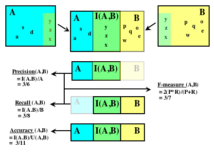
The descriptions of term set shape described above are useful in that they can be applied to any set of terms independently and because they provide detailed descriptions of the term sets, but, from the perspective of comparison, more direct methods are also applicable. To provide a more exact comparison of the compositions of sets of terms used in different languages, we suggest several simple measures of set similarity. Each of the measures is a view on the relation between the size of the intersection of the two term sets and the relative sizes of each set. The members of the intersection are determined through exact string matches applied to the term sets (after a series of syntactic normalization operations). As depicted in Figure 1 and explained below, these intersections are used to produce measures of precision, Recall, and Overlap (the F-measure).

Context considerations in inter-set comparisons

The equivalence function used when conducting direct set comparisons of the components of different indexing languages is important. In this preliminary work, we rely on the simplistic notion that a term in one indexing language is equivalent to a term in another language if and only if, after syntactic normalization, the terms are identical. Synonymy, hyponymy and polysemy are not considered and, thus, the measured overlaps are purely syntactic. When considering indexing languages used in similar contexts; for example, as might be indicated when two different languages are used to index the same set of documents by similar groups of people, this function provides useful information because the same words are likely to be used for similar purposes. However, the greater the difference in context of application between the indexing languages being compared, the greater the danger that this simple function will not yield relevant data. Logical extensions of this work would thus be to make use of semantic relations, for example of synonymy, present within the indexing languages, as well as natural language processing techniques, to develop additional equivalence functions that operate on a more semantic level. That being said, with or without such extensions, any empirical comparison should always be interpreted in light of the contexts within which the different indexing languages operate.

Quantifying set similarity

Once methods for assessing the equivalence relationship are established (here post-normalization string matching), it is possible to quantify the relations between the resultant sets in several different ways. For example, Al-Khalifa and Davis (2007) find what they term percentage overlap by dividing the size of the intersection of the two sets by the size of the union of the sets and multiplying by 100. They use this measure to quantify the similarity of the sets of terms used to index the same documents produced by different indexing systems. For example, to find the percentage overlap between the set F {A,B,C} and the set K{A,G,K,L} , the size of the intersection {A} is 1, the size of their union {A,B,C,G,K,L} is 6 and thus the percentage overlap is 100(1/6)= 17%.

While a useful measurement, this equation misses key information regarding the relative sizes of the two sets. To capture the size discrepancies and the asymmetry of the relationship, we employ additional metrics typically used to evaluate class prediction algorithms.

Binary class prediction algorithms are often evaluated on the basis of relations between sets of true and false positive and negative predictions (Witten & Frank 2000). These relations are quantified with measures of Accuracy, precision and Recall. Accuracy is the number of correct predictions divided by the number of false predictions. precision is the number of true positives divided by the number of predicted positives. Recall is the number of true positives divided by the number of both true and false positives. precision and Recall are often summarized with the F-measure, which equates to their harmonic mean.

Hripcsak and Rothschild (2005) showed that, by arbitrarily assigning one set as the true positives and the other as the predicted positives, the F-measure can be used to measure the degree of agreement between any two sets. Because it is commutative, the choice of which set to assign as true makes no difference to the outcome. Figure 1 illustrates the idea of using precision, Recall, and the F-measure as generic set comparison operators. The logic goes as follows, if set A is conceptualized as an attempt to predict set B, the number of items in both sets (the intersection) corresponds to the number of true positives for the predictor that produced A; the number of items in A corresponds to the number of true positives plus the number of false positives; and the number of items in B corresponds to the number of true positives plus the number of false negatives. From this perspective, accuracy thus equates to percentage overlap as described by Al-Khalifa and Davis (2007). In addition, precision and Recall can be used for the asymmetric quantification of the similarity of the two sets and the F-measure can be used to provide a symmetric view of the overlap between the sets that takes into account their relative sizes.

Demonstration and evaluation of proposed metrics

The metrics described above are intended to be useful in scientific enquiries regarding the relationships that hold between different indexing languages. This information, in turn, should then be useful in informing assumptions about the relationships between the information systems that generate and use these languages. As such, it should be possible to use the metrics to answer specific questions. We chose the following questions as demonstrative examples:

1. Are the intra-set characteristics of the folksonomies emerging from collaborative tagging systems sufficient to distinguish them from term sets associated with indexing languages created using professional labour? (We assume that the difference in kind between these groups will be expressed in a difference in shape as expressed in the intra-set measures.)
2. How much direct overlap exists between terms from the Connotea, Bibsonomy, and CiteULike folksonomies, and terms from MeSH? These folksonomies are used to describe tens of thousands of the same resources as MeSH, hence we expect some overlap in representation, but how much is there in reality?

To answer these questions and thus demonstrate example applications of the proposed set of metrics, we implemented programs that calculate each intra- and inter-set metric described above. In the text that follows, we describe the application of these programs to the automated characterization and comparison of twenty-two different indexing languages.

Sample

We gathered a sample of twenty-two different term sets. The terms were extracted from folksonomies, thesauri, and ontologies, all of which are currently in active use. Our domains span biology, medicine, agriculture, and computer science; however, the sample set is biased towards biology and medicine. Ontologies constitute the most common type of structure in the sample simply because more of them were accessible than the other forms, Table 4 lists the subjects of the study (note that there are more than twenty-two listed because multiple versions for some of the larger term sets were considered separately).

The indexing languages considered here were chosen for three general reasons: (1) they were freely available on the Web, (2) most of the terms associated with the indexing languages had representations in English and (3) we sought popular examples spanning both controlled and uncontrolled indexing languages. Availability on the Web not only made data collection for the present study easier, it increases the likelihood that the study could be repeated by others in the future. By constraining the natural language of origin for the indexing languages under study, the likelihood that the measured differences between term sets were the results of factors aside from differences in, for example, typical grammatical structure of the source languages, was increased. Finally, by sampling from a broad range of the known types of indexing language, as suggested, for example, in the typology of Tudhope (2006), we hoped to show the generic nature of the metrics introduced here and to offer some basic exploratory comparisons of the broad groups of controlled and uncontrolled languages.

Although we provide results for all of the inter-term set comparisons, the emphasis of the set comparisons is on the relationship between MeSH and the uncontrolled indexing languages. To partially decrease the problems, noted above, associated with conducting syntactic comparisons of indexing languages operating in different contexts, uncontrolled languages were sought that were used to index many of the same documents as MeSH. Folksonomies emanating from social tagging services targeted towards academic audiences thus compose the set of uncontrolled languages in the sample.

Data analysis

Once each of the term sets was collected (see Appendix 1), two levels of term normalization were applied corresponding to the intra-set analysis (phase 1) and the inter-set analysis (phase 2). Both phases were designed based on the premise that most of the terms in the structures were English words. Though there were certainly some non-English terms present in the folksonomy data, notably German and Spanish, these terms constituted a relatively small minority of the terms in the set and, as such, we do not believe they had any significant effect on the results.

Phase 1 term normalization

Phase 1 normalization was designed primarily to help consistently delineate the boundaries of compound words, especially in the case of the folksonomies. The operations were:

1. All non-word characters (for example, comma, semi-colon, underline and hyphen) were mapped to spaces using a regular expression. So the term automatic-ontology_evaluation would become automatic ontology evaluation.
2. CamelCase compound words were mapped to space separated words: camelCase becomes camel case.
3. All words were made all lower case (case-folded).
4. Any redundant terms were removed such that, after operations 1-3, each term in a set composed a string of characters that was unique within that set.

All of the intra-set measurements (Size and Flexibility for example) were taken after Phase 1 normalization. Phase 2 normalization was applied before the set-intersection computations (for the inter-set measurements).

Phase 2 term normalization

Phase 2 normalization was intended to reduce the effects of uninformative inconsistencies such as dolphins not matching dolphin when estimating the intersections of the term sets.

1. Phase 1 normalization was applied.
2. Porter stemming was applied to all terms and sub-terms (Porter 1980).
3. All sub-terms were sorted alphabetically.
4. All terms and sub-terms with less than two characters were removed.
5. All terms and sub-terms matching words from a popular English stop-word list were removed (Default... 2008)

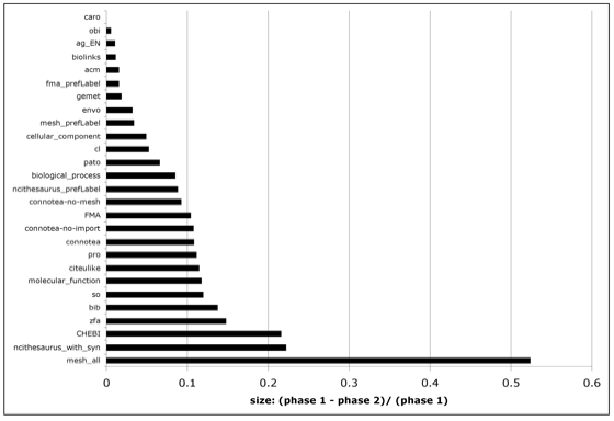
These additional steps resulted in an average reduction in the total number of distinct terms per term set of 13% with the most substantial difference seen for the MeSH all term set, which included both the preferred labels for each descriptor and all of the alternate labels, at 52%. The set of just the preferred labels for the MeSH descriptors was only reduced by 3%. This demonstrates that the normalization step was successful in reducing redundancy within the term sets because the MeSH all set intentionally includes many variations of the same term while the preferred labels are intended to be distinct. Figure 2 plots the reduction in the (non-redundant) term set size between phase 1 and phase 2 normalization for all the term sets.

Figure 2: The effect of phase 2 normalization on the size of the term set
(For each term set, the chart displays the ratio of its size after phase 2 normalization versus its size after phase 1 normalization.)

After normalization, the shape of each of the term sets was first assessed individually using the intra-set measures. Then each of the term sets was compared directly to all others using the inter-set metrics.

Intra-set findings

The intra-set measures displayed a broad range of diversity across all of the samples and provided some preliminary evidence of the presence of distinct shapes associated with term sets originating from controlled versus uncontrolled information organization structures. The collected measurements are provided in Tables 5 to 7 and discussed below.

Table 5 contains the non-ratio measurements of the size and the composition of the term sets. From it, we can see that there is a wide range in the size and degrees of modularity of the term sets under study. The largest term set was the CiteULike folksonomy at 234,223 terms and the smallest was the Common Anatomy Reference ontology (Haendel et al. 2008) at just fifty terms. There was also substantial variation in the total number of Observed Linguistic Precoordination sub-terms per term, with the CHEBI ontology (Degtyarenko et al. 2008) averaging 8.88 while the Bibsonomy folksonomy averaged just 0.63. This is suggestive of differences in the relative compositionality of the different term sets, with the ontologies being much more modular in general than the folksonomies.

The sub-terms per term measurement highlights the uniqueness of the CHEBI ontology within the context of our sample; its terms include both normal language constructs like tetracenomycin F1 methyl ester and chemical codes like methyl 3,8,10,12-tetrahydroxy-1-methyl-11-oxo-6,11-dihydrotetracene-2-carboxylate. Although both term structures are highly modular in this large ontology, the latter are clearly driving the very high observed mean number of sub-terms per term.

Table 6 focuses specifically on illustrating the amount of modularity apparent in these term sets. It displays the percentages of uniterms, duplets, triplets, and quadplus terms; the flexibility, and the percentages of terms that contain other terms or are contained by other terms. The CiteULike folksonomy has the highest percentage of uniterms at 75.8%, followed closely by the Bibsonomy folksonomy at 72.7%, while the two lowest percentages are observed for the Foundational Model of Anatomy (FMA) (including synonyms), described by Rosse and Mejino (2003), at 1.2% and the Biological Process (BP) branch of the Gene Ontology, described by Ashburner et al. (2000) at 0.8%. This tendency towards increased compositionality in these ontologies and decreased compositionality in these folksonomies is also apparent in the percentage of their terms that contain other complete terms from the structure, with more than 95% of the FMA terms containing other FMA terms and only 23.8% of the Bibsonomy terms containing another Bibsonomy term. As might be expected, larger average term lengths, as presented in Table 7, appear to correlate to some extent with some of the measures indicating increased compositionality. The highest correlation for a compositionality measure with average term length was observed for Observed Linguistic Precoordination Quad Plus (r-squared 0.86) while the lowest was for containedByAnother (r-squared 0.13). The highest mean term length observed was 40.35 characters for the preferred labels for the FMA and the lowest was 10.19 for the Bibsonomy terms.

Factor analysis

Following the collection of the individual parameters described above, exploratory factor analysis was applied to the data to deduce the major dimensions. Before executing the factor analysis, the data were pruned manually to reduce the degree of correlation between the variables. The features utilized in the factor analysis were thus limited to percent of uniterms, percent of duplets, percent of quadplus, flexibility, percent of containsAnother, percent of containedByAnother, mean number of sub-terms per term, mean term length, and the coefficient of variation for term length. Maximum likelihood factor analysis, as implemented in the R statistical programming environment by the R Development Core Team (2008), was applied using these variables for all of the sampled term sets. Three tests were conducted with 1, 2, and 3 factors to be fitted respectively. In each of these tests, the dominant factor, which might be labelled term complexity, was associated with the variables: percent of quadplus, mean term length, and mean sub-terms per term. In the 2-factor test, the secondary factor was most associated with the percent of uniterms and the flexibility. Finally, in the 3 factor analysis, the third factor was associated with percent of containsAnother and percent containedByAnother. Table 8 provides the factor loadings for the 3-factor test.

Controlled versus uncontrolled term sets

The data presented in Tables 5 to 7 provide evidence that the metrics captured here are sufficient to distinguish between term sets representing different indexing languages. To assess their utility in quantifying differences between indexing languages emanating from different kinds of information system, we tested to see if they could be used to differentiate between the languages produced by professional labour (the thesauri and the ontologies) and languages generated by the masses (the folksonomies).

This examination was conducted using manual inspection of the data, multi-dimensional visualization, and cluster analysis. At each step, we tested to see if the data suggested the presence of a distinct constellation of intra-set parameters associated with the term sets drawn from the folksonomies. For some subsets of variables, the difference was obvious. For example, as Figure 3 illustrates, both the percent of uniterms and the Observed Linguistic Precoordination flexibility measurements were sufficient to separate the folksonomies from the other term sets independently. For other subsets of variables, the differences were less clear and, in some cases, the folksonomies did not group together.

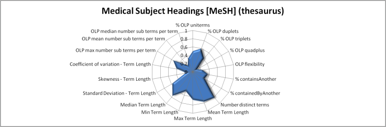
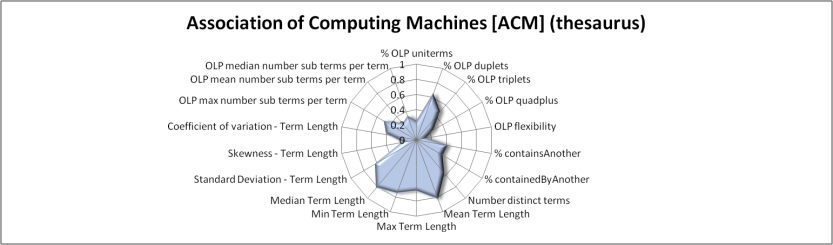
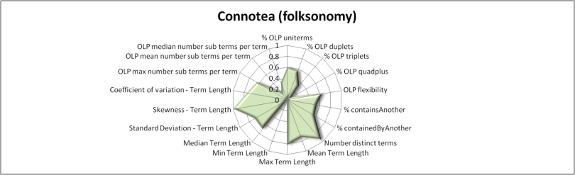
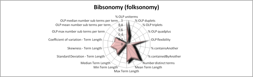
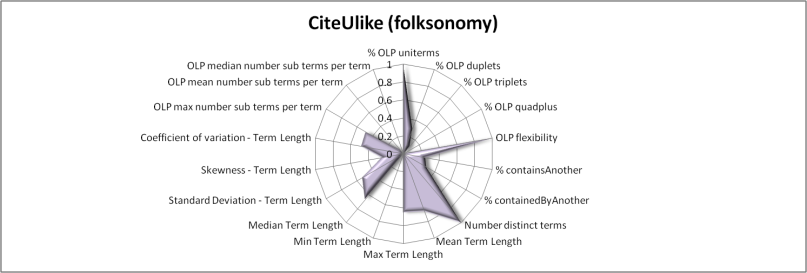
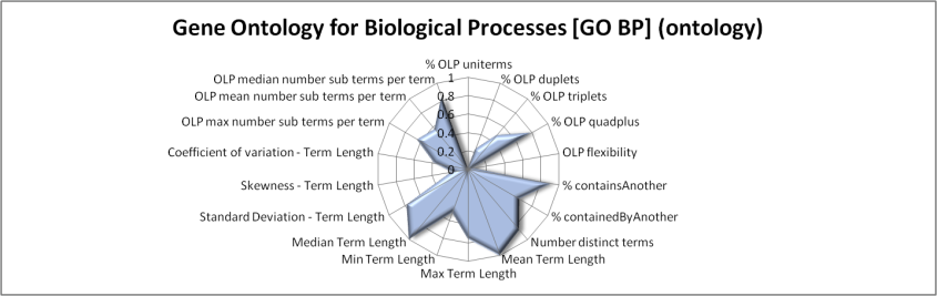
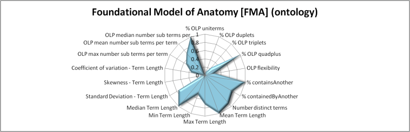
Figures 4 to 10 use radar-charts to illustrate the shapes associated with the three folksonomies in the sample as well as representative ontologies and thesauri. Radar charts were chosen because they make it possible to visualize large numbers of dimensions simultaneously. Though it would be possible to reduce the number of features in the charts, for example using the results from the factor analysis presented above, we chose to present all of the measurements taken. These figures, which capture all of the features measured for a given term set in a single image, suggest fairly distinct patterns in the term sets associated with the different kinds of information system present in our sample. However, when utilizing all of the variables, the borders of the various categories are not entirely clear. For example, the Bibsonomy and CiteULike folksonomies appear to be nearly identical in these charts but, while similar, the Connotea folksonomy shows substantial variations.

In various iterations of cluster analysis we repeatedly found that the Bibsonomy and the CiteULike term sets grouped tightly together and that Connotea was generally similar to them but that this similarity was strongly influenced by the specific subset of the metrics used. In one specific analysis presented in Good & Tennis (2008), Ward’s method identified a distinct cluster containing just the folksonomies using the following parameters: percent of uniterms, percent of duplets, flexibility, percent contained by another, standard deviation of term length, skewness of term length, and number of complements.

Figure 3: %Uniterms verse Observed Linguistic Precoordination flexibility
(Either metric is sufficient to form a linear separator between the term sets originating from folksonomies (the three in the upper right corner) and the controlled terms from the other information organization structures in the sample. The Pearson correlation coefficient for percent of uniterms and Observed Linguistic Precoordination flexibility is 0.79. )

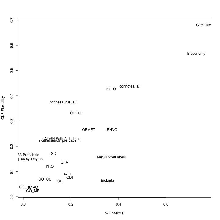
These results indicate that the answer to the first question, namely: Are the terms from folksonomies shaped differently than the terms from controlled vocabularies? is, generally, yes. Subsets of these metrics can be used to separate folksonomies from the controlled vocabularies using a variety of methods. However, Bibsonomy and CiteULike are clearly much more similar to each other than either is to Connotea. Without advancing a definitive answer as to why this is the case, we offer several possible explanations. First, one clear technical difference between Connotea and the other two systems is that it allows spaces in its tags. For example, it is possible to use the tag semantic Web in Connotea, but, in Bibsonomy or CiteULike, one would have to use a construct like semanticWeb, semantic-Web, or semanticWeb to express the same term. Though the syntactic normalization we utilized will equate semantic-Web with semantic Web (and detect the two-term composition), the term semanticWeb would not match and would be classified by the system as a uniterm. This difference suggests that there may be more compound terms in Bibsonomy and CiteULike than our metrics indicate; however, this aspect of the tagging system may also act to discourage the use of complex tags by the Bibsonomy and CiteULike users. Aside from differences in the allowed syntax of these uncontrolled indexing languages, this may also be an effect of the differing communities that use these systems. While Connotea is clearly dominated by biomedical researchers, Bibsonomy is much more influenced by computer scientists and CiteULike seems to have the broadest mixture. Perhaps the biomedical tags are simply longer and more complex than in other fields. A final possibility, one that we will return to in the discussion of the direct measures of term-set overlap, is that Connotea may be disproportionately affected by the automatic import of terms from controlled vocabularies, in particular MeSH, as tags within the system.

Figure 4: Radar graph of the MeSH thesaurus

Figure 5: Radar graph of the Association for Computing Machinery (ACM) thesaurus

Figure 6: Radar graph of the Connotea folksonomy

Figure 7: Radar graph of the Bibsonomy folksonomy

Figure 8: Radar graph of the CiteULike folksonomy

Figure 9: Radar graph of term set from Gene Ontology Biological Process (GO_BP)

Figure 10: Radar graph of term set from the Foundational Model of Anatomy (FMA)

Inter-set findings

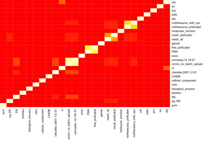
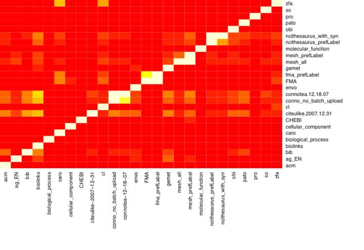
Following the intra-set results, the inter-set comparisons indicate high diversity in the term sets present in the sample while also highlighting interesting relationships between them. Figures 11 and 12 provide an overview of the all-against-all comparison of each of the term sets using the F-measure and the measures of precision and recall respectively. They show that, in general, there was a very low amount of overlap between most of the pairs that were examined. This is likely a direct result of the wide variance of contexts associated with the diverse indexing languages represented in the sample. Though the sample was biased towards ontologies in the biomedical domain, biomedical is an extremely broad term. For example, the domains of items intended to be indexed with the different languages ranged from amino acid sequences, to biomedical citations, to tissue samples. That there was not much direct overlap in general is unsurprising.

Aside from overlaps between different term sets drawn from the same structure (e.g., between a version of MeSH with only the preferred labels and a version that included all of the alternate labels), the greatest overlap, as indicated by the F-measure, was found between the Zebrafish Anatomy (ZFA) ontology (Sprague et al. 2008) and the Cell ontology (CL) (Bard et al. 2005) at (f = 0.28). This overlap results because the ZFA ontology contains a large proportion of cell-related terms that are non-specific to the Zebrafish, such as mesothelial cell and osteoblast.

Table 9 lists the F-measure, precision and recall estimates for the term-set pairs with the highest F-measures. Aside from the ZFA/CL comparison, the greatest overlaps were observed for the inter-folksonomy pairs, MeSH and the Agricultural Information Management Standards thesaurus (Ag), MeSH and the National Cancer Institute thesaurus (NCI) (Sioutos et al. 2007), and MeSH and Connotea (Lund et al. 2005).

MeSH versus the folksonomies

The second specific, demonstrative question put forward above, and one of the early motivators for this project, was the question of how the terms from MeSH compare to the terms from academic folksonomies. To answer this question, Tables 10 and 11 delineate the overlaps in terms of precision, recall, and the F-measure that were observed between the three folksonomies in our sample and the MeSH thesaurus (including one version with just the preferred labels and another that included alternate terms). Of the three folksonomies, Connotea displayed the greatest degree of overlap with MeSH in terms of the F-measure, precision, and recall for both the preferred labels and the complete MeSH term set. The precision of the Connotea terms with respect to the MeSH preferred labels was 0.073, the recall 0.363, and the F-measure was 0.122.

The fact that the Connotea term set contains nearly 9000 MeSH terms (36% of the entire set of preferred labels) suggests a) that there are a number of biomedical researchers using Connotea and b) that they have chosen, one way or another, to utilize MeSH terminology in the organization of their publicly accessible resource collections. How these terms came to be used in this manner is a more difficult question. In some cases, the Connotea users likely recreated the MeSH terms when going about their normal tagging practices; however, the relatively high level of overlap is suggestive of other underlying factors.

Batch import in folksonomies

Connotea, as well as the other social tagging systems in the study, offers a way to import data from other sources automatically. For example, it is possible to export bibliographic information from applications such as Endnote and then import these records as bookmarks within the Connotea system. This opens up the possibility that tags generated outside of the Connotea system, such as MeSH indexing by MEDLINE, can wind up in the mix of the tags contained within the Connotea folksonomy.

To help assess the impact of imported tags on the contents of the Connotea folksonomy, we identified and removed a subset of the Connotea tags that were highly likely to have been imported through the use of additional information about the context of the creation of the tags, and then recomputed all of the metrics defined above. In a social bookmarking system like Connotea, tags are added to the system as descriptive annotations of Web resources. When a bookmark is posted to the system by a particular user, the tags associated with it, as well as a timestamp, are associated with the entry. Sets of bookmarks posted via batch import, for example from the contents of an Endnote library, will all have nearly identical timestamps associated with them. Thus, by pruning out tags originating only in posts submitted by the same user during the same minute, we constructed a new Connotea term set that should be more representative of the terms actually typed in directly by the users.

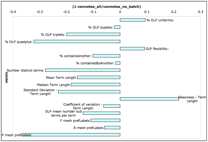
Figure 13 shows the differences between the pruned Connotea term set (Connotea_no_batch) and the original dataset on both intra-set measures and measures of direct overlap with the MeSH preferredLabel term set. In every metric except for the skewness of the lengths of the terms, the pruned Connotea term set more closely resembled the other folksonomies. For example, in the pruned set, the % uniterms increased by about 10%, the % quadplus decreased by more than 30% and the flexibility increased by about 10%. The overlap with the MeSH prefLabels decreased from 0.12 to 0.11 with respect to the F measure, the precision decreased from 0.363 to 0.266, and the recall decreased from 0.073 to 0.069.

Figure 13: Differences between the full Connotea term set and Connotea term set with batch uploaded bookmark posts removed

It appears the process of batch uploading bookmarks in Connotea, in cooperation with other personal information management practices such as the use of Endnote, has influenced the contents of the Connotea folksonomy. In particular, many MeSH terms appear to have been incorporated into it. Since most other folksonomies, including the others evaluated here, also have automated upload capabilities, it is highly likely that similar results may be observed within them. While this phenomenon makes the interpretation of folksonomy datasets more complex by obscuring the origins of the data, its illumination should provide new opportunities for investigation. For example, perhaps it would be possible to track the migration of terms across the boundaries of different systems through the addition of a temporal attribute to the inter-set metrics suggested here. Such data might help to explain the origins of the terms utilized in different indexing languages. One would assume for example, that many of the terms that now overlap between MeSH and the folksonomies appeared first in MeSH and then migrated over somehow; however, in the future, perhaps this process might be reversed as folksonomies are mined for candidate extensions to controlled vocabularies.

Discussion

Robust, reproducible methods for comparing different information systems are vital tools for scientists and system developers faced with what has been called ‘an unprecedented increase in the number and variety of formal and informal systems for knowledge representation and organization’ (Tennis & Jacob 2008). Indeed, we are in a Cambrian Age of Web-based indexing languages. Metrics and tools, such as the system for indexing language characterization described here, can be used to provide information about how the many emerging kinds of information systems relate to one another. It can also be used in the design of new systems that incorporate ideas inspired by such comparisons, as suggested by the University of California’s Bibliographic Services Task Force (2005), or, as demonstrated by Good et al. (2006) and Willighagen et al. (2007), explicitly combine multiple extant systems to form novel hybrids.

In the research presented above, we introduced metrics for the automatic characterization and set-theoretic comparison of sets of terms from indexing languages. Using these metrics, we provided a broad-spectrum analysis of twenty-two different languages. Within the data gathered in this exploratory analysis, we identified suggestive patterns associated with the terms that compose folksonomies versus the terms from controlled vocabularies as well as directly quantifying the degree of overlap present across each of the sets in the sample. Of particular interest is the apparent migration of terms across the boundaries of the different systems, in particular from MeSH into the folksonomies. Though the results presented here are informative, the main contribution of this work is the enumeration and implementation of the comparative protocol.

Future term set analyses, particularly if they can be integrated with rich qualitative dimensions, might be put to any number of novel uses. Given the definition of these metrics and the provision of tools for their calculation, it would now be straightforward to test whether any of the term-based measurements are related to other attributes of information systems. For example, it might be interesting to test to see if any of these factors were predictive of system performance; e.g., is the percentage of uniterms in the tags that compose a folksonomy correlated with the performance of that folksonomy in the context of a retrieval task? If that answer turned out to be yes, then it would offer an easy way to estimate the retrieval performance of different systems and might suggest ways to improve performance, for example by adapting the tagging interface to encourage the contribution of more complex tags. Other potential applications include: comparative quality evaluation, term set warrant and the identification of relationships between term-set shape and theoretical types of indexing language.

Comparative quality evaluation

From the perspective of systems evaluation, one particular use of the methods defined here might be in gold-standard based quality assessments similar to those described by Dellschaft and Staab (2006) for the automated, comparative evaluation of ontologies. If a particular indexing language is judged to be of high quality for some particular context, other structures might be evaluated for their quality in that or a very similar context based on their similarity to this gold-standard. For example, for the purpose of indexing biomedical documents for an institutional information retrieval system like MEDLINE, many would consider MeSH as a gold standard. The similarity of another indexing language, such as a folksonomy, to this standard might thus be used as a measure of its quality for indexing biomedical documents for retrieval. The principle advantage of such an approach is that it can be completely automatic, potentially helping to avoid the intensive manual labour and possible subjectivity associated with manual evaluations. The disadvantages are that, for any real, new application, (a) a gold standard is unlikely to exist and (b) any acceptable evaluation would still have to be informed by extensive qualitative alignment of the contextual attributes of the intended application in comparison with the gold standard.

Term-set warrant

The creators and maintainers of indexing languages often require justifications for the inclusion or exclusion of classes within their structures (Beghtol 1986: 110-111). These justifications, referred to as warrants, may come in many forms, though the most commonly discussed is probably literary warrant. Essentially a particular kind of warrant bases the justification for the contents of an indexing language on a particular kind of empirical evidence (e.g., user requests) or argument (e.g., philosophical or scientific warrant). The inter-set metrics may provide data useful in the development of a new kind of warrant based upon the overlap between different structures. Essentially, such a term-set warrant might be invoked to justify the inclusion of terms or the concepts they represent based on the presence or absence of those terms in other structures.

Relationship of term-set shape to theoretical type

It is tempting to think that this approach, or some extension of it, could be used to describe meaningful types of indexing languages, not from design requirements, but from the actualization of those design requirements manifest in and observable to us in the shape of term sets. This could provide a weak empirical corroboration for types of indexing languages in use, not only according to standard or theory, but based on empirical evidence of term corpus. Defending and making use of such inferences would require a solid understanding of the meaning of the different shapes. The work presented here is exploratory and future work will have to substantiate any claim at deriving type from these empirical factors. However, we can see that, in this sample, there were clear distinctions between the shapes of controlled and uncontrolled vocabularies, demonstrating at this stage that we can hypothesize that folksonomies have a particular shape in relation to both thesauri and ontologies. Future studies may take advantage of the increasing number of different indexing languages to, for example, attempt to define the relationship of term-set shape to the breakdown of theoretical type within the controlled vocabularies.

Future work

The metrics derived and applied here operate at what amounts to a syntactic level and no specific attempt, other than rudimentary term normalization, was made to identify the concepts present in the different indexing languages. A natural extension of this work would be to apply natural language processing technology to make this attempt. The rough indications of semantic similarity provided by the inter-term set comparisons could be made much more robust if the comparisons were made at the level of concepts rather than terms, for example making it possible to equate synonymous terms from different languages.

Aside from the incorporation of natural language processing technology for concept identification, it would be useful to consider the analysis of predicate relationships between the terms (e.g., the hierarchical structure) and the analysis of the relationships between terms and the items they may be used to index. Metrics that captured these additional facets of information systems, characteristic of their form and application, would provide the opportunity for much more detailed comparisons, thus forming the raw materials for the derivation and testing of many new hypotheses.

There remain many indexing languages, both controlled and uncontrolled, that are available online that have not been characterized with the methods and from the naturalistic perspective adopted here. In addition to improving and expanding methods, the majority of future work will be the application of these tools to the analysis of other languages.

Conclusion

We are at the very beginning of a rapid expansion in the number and the diversity of different frameworks for the organization of information. As more and more information systems come into the world, the application of expository, reproducible protocols for their comparative analysis, such as the one described in this article, will lead to ever increasing abilities to illuminate and thus build upon this expanding diversity of form and content.

Note

Availability. All materials, including the programs generated to conduct the term set analysis and the term sets analysed, are freely available at http://biordf.net/~bgood/tsa/.

Acknowledgements

B.M. Good is supported by a University of British Columbia Graduate Student Fellowship.

About the authors

Joseph T. Tennis is an Assistant Professor at the Information School of the University of Washington, Associate Member of the Peter Wall Institute for Advanced Study at The University of British Columbia, and Reviews Editor for Knowledge Organization. He is also a member of the Dublin Core Usage Board. He received his M.L.S. from Indiana University and the Ph.D. in Information Science from the University of Washington. He works in classification theory, the versioning of classification schemes and thesauri (subject ontogeny), and the comparative discursive analysis of metadata creation and evaluation, both contemporary and historical. He can be contacted at jtennis@u.washington.edu

Benjamin M. Good is a Ph.D. candidate in Bioinformatics at the University of British Columbia. He received his M.Sc. in Evolutionary and Adaptive Systems from the University of Sussex and his B.Sc. in Cognitive Science from the University of California at San Diego. His current research focuses on the design of mass-collaborative strategies for building and automated methods for characterizing the content of the semantic Web. He can be contacted at: goodb@interchange.ubc.ca

Bookmark This Page

Appendix 1. Data collection: assembly of term sets

MeSH

1. Files representing the 2008 release of MeSH were downloaded from http://www.nlm.nih.gov/mesh/filelist.html on 11 February 2008.
2. The preferred labels for the terms were taken from the downloaded file 'mshd2008.txt'.
3. The union of the preferred labels and the synonyms (mesh all) was extracted from the downloaded MeSH XML file 'desc2008' using a Java program.
4. The MeSH terms with comma separated adjectives, like 'Cells, Immobilized', were programmatically re-ordered to reflect a more natural English language usage of adjective-noun, such as 'Immobilized Cells'. This step was taken to facilitate comparison with the other indexing languages that tended much more towards this form.

OWL/RDF formatted thesauri and ontologies

Unless otherwise, noted, all the labels for the concepts and their synonyms were extracted from the files using custom Java code built with the Jena OWL/RDF API.

ACM – Association for Computing Machinery

An OWL-XML version of the 1998 ACM thesaurus was acquired from Miguel Ferreira of the Department of Information Systems at the University of Minho.

AG – AGROVOC thesaurus from the Agricultural Information Management Standards initiative

An OWL-XML file containing the thesaurus ('ag_2007020219.owl') was downloaded from http://www.fao.org/aims/ag_download.htm

BioLinks

BioLinks is a subject listing used to organize the bioinformatics links directory. An OWL version of these subject headings was composed by one of the authors in August of 2007, and is available at http://biordf.net/~bgood/ont/BioLinks.owl.

Open Biomedical Ontologies (OBO)

The daily OWL versions of the following ontologies from the OBO foundry were downloaded from http://www.berkeleybop.org/ontologies/ on 11 February 2008.

• Gene Ontology (biological process, molecular function, cellular component)
• CARO – common anatomy reference ontology
• CHEBI – chemical entities of biological interest
• CL – cell ontology
• ENVO – environment ontology
• FMA – an OWL version of the Foundational Model of Anatomy
• NCI Thesaurus – National Cancer Institute thesaurus
• OBI – Ontology for Biomedical Investigations
• PATO – Phenotypic Quality ontology
• PRO – Protein Ontology
• SO – Sequence Ontology
• ZFA – Zebrafish Anatomy and Development Ontology

GEMET

GEMET - the thesaurus used by the European Environment Information and Observation Network - was downloaded from http://www.eionet.europa.eu/gemet/rdf?langcode=en on 15 February 2008. The English terms were extracted from the provided HTML table.

Folksonomies (collections of tags created in social bookmarking systems)

• Connotea
  The Connotea folksonomy was extracted from 377885 posts to Connotea collected prior to 12 December 2007. The Connotea Web API and the Connotea Java library were used to gather and process the data.
• Bibsonomy
  The Bibsonomy tag set was extracted from a 1 January 2008 export of the Bibsonomy database. It is available for research upon request from Webmaster@bibsonomy.org.
• CiteULike
  The CiteULike tag set was extracted from a 31 December 2007 export of the CiteULike database. Daily versions of this database are available for research purposes from http://www.citeulike.org/faq/data.adp.

Hit Counter by Digits

® the authors, 2009. Last updated: 2 March, 2009

online Web site analytics